Create colorful contour maps with custom levels, colors, and a color scale!
Contour Map Features
- Automatic or user-defined contour intervals and ranges
- Full control over contour label format, font, frequency, placement, and spacing
- Drag contour labels to place them exactly where you want them
- Automatic or user-defined color for contour lines
- Color fill between contours, either user-specified or as a custom color map of your choice
- Save and load custom color map files for the exact desired display
- Use one of the built-in presets as the color map
- Full control over hachures
- Save and load contour map level files that contain all the level information, so you can easily and quickly create contour maps with consistent properties
- Regulate smoothing of contour lines
- Blank contour lines in areas where you don't want to show any data
- Specify color for blanked regions, or make them transparent
- Add color scale
- Create any number of contour maps on a page
- Add base, vector, shaded relief, image, or post map layers to contour map layers
- Drape contour map layers over 3D surfaces or 3D wireframes for dramatic displays
- Export contours in 3D DXF and 3D SHP formats
- Adjust the layer opacity
Individual contour labels can be dragged to a new location,
new labels can be added and individual labels can be deleted.
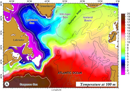
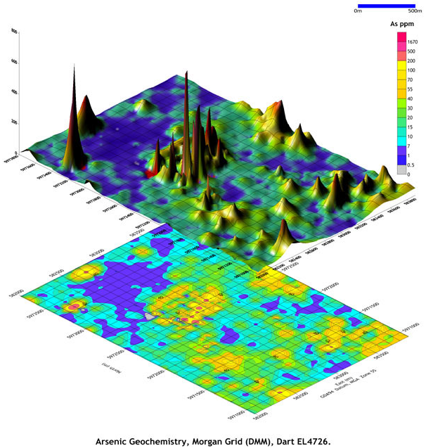
Create vibrant and informative contour maps and overlay them with post maps of the original data points!
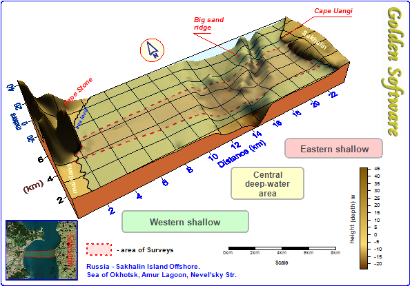
3D Surface Maps
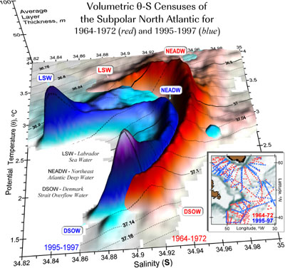
The 3D surface map uses shading and color to emphasize your data features. Change the lighting, display angle and tilt with a click of the mouse. Overlay several surface maps to generate informative block diagrams.
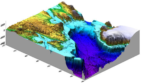
Create exciting 3D surface maps from your XYZ data!
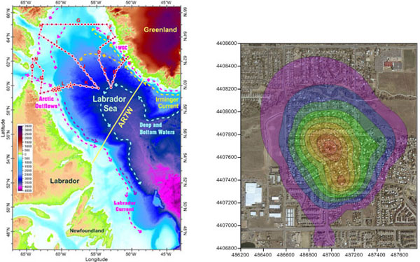
Image courtesy of Igor Yashayaev, Bedford Institute of Oceanography, Fisheries and Oceans, Canada.
3D Surface Map Features
- Specify surface color gradation, shininess, base fill and line color
- Control mesh line frequency, color, style, surface offset
- Set lighting horizontal and vertical angles, ambient, diffuse, and specular properties
- Overlay contour maps, image maps, post maps, shaded relief maps, raster and vector base maps, and other surface maps for spectacular presentations
- Choose overlay resample method and resolution, color modulation (blending) of surface and overlays
- Save and load custom color map files for the exact desired display
- Use one of the built-in presets as the color map
- Add color scales to explain the data values corresponding to each color
- Disable the display of blanked grid nodes or map the blanked areas to a specific Z level
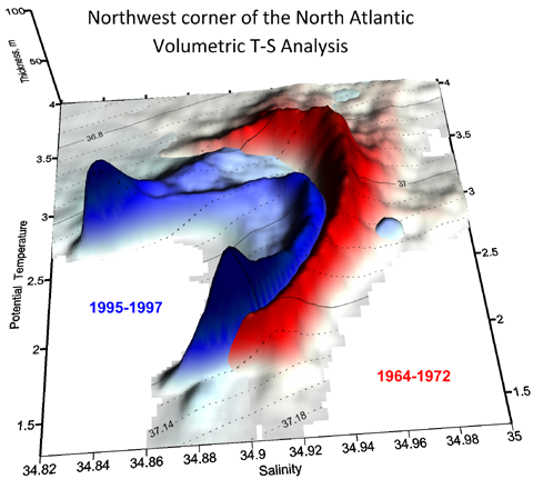
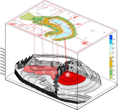
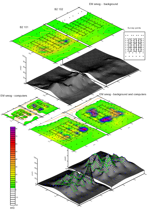
Combining surface maps is an excellent technique to visually compare data sets.
Image courtesy of Igor Yashayaev, Bedford Institute of Oceanography, Fisheries and Oceans, Canada.
Overlay surface maps to visually depict changes with depth!
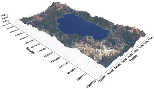
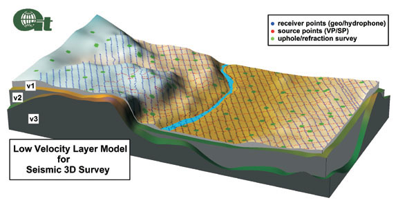
Create photo-realistic 3D models containing both terrain and ground cover detail by
overlaying 3D surfaces with aerial photography, satellite imagery or other images.
Image Maps
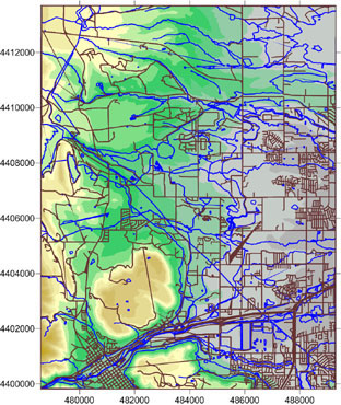
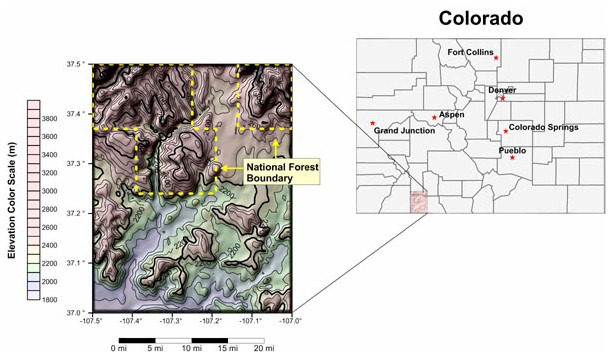
Surfer image maps use different colors to represent elevations of a grid file. Surfer automatically blends colors between percentage values so you end up with a smooth color gradation over the entire map. You can add color anchors at any percentage point between 0 and 100. Each anchor point can be assigned a unique color, and the colors are automatically blended between adjacent anchor points. This allows you to create color maps using any combination of colors. Add a color scale to show the values of the different colors! Image maps can be created independently of other maps, or can be combined with other map layers. They can be scaled, resized, limited and moved.
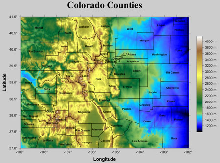
Customize your image map by adding color, including a color scale, and
overlaying it with other map layers to make the map as informative as
possible! The above map is created from an image map of Colorado
elevation overlaid with a base map layer showing the county boundaries.
Image Map Features
- Display pixel maps or smoothed images
- Save and load custom color map files for the exact desired display
- Use one of the built-in presets as the color map
- Create an associated color scale
- Overlay image maps with contour, post, or base maps
- Specify a color for missing data, or choose to make areas of no data transparent
- Change the rotation and tilt angles
- Adjust the layer opacity
Colorful and smooth image maps can be combined with base maps and
contour maps to create informative displays. Image courtesy of Igor
Yashayaev, Bedford Institute of Oceanography, Canada.
Shaded Relief Maps
Shaded relief maps are raster images based on grid files. Shaded relief maps assign colors based on slope orientation relative to a light source. Surfer determines the orientation of each grid cell and calculates reflectance of a point light source on the grid surface.
The light source can be thought of as the sun shining on a topographic surface. Surfer automatically blends colors between percentage values so you end up with a smooth color gradation over the map. You can add color anchors so each anchor point can be assigned a unique color, and the colors are automatically blended between adjacent anchor points. This allows you to create color maps using any combination of colors. Shaded relief maps can be created independently of other maps, or can be combined with other layers. Shaded relief maps can be scaled, resized, limited, and moved in the same way as other types of maps.
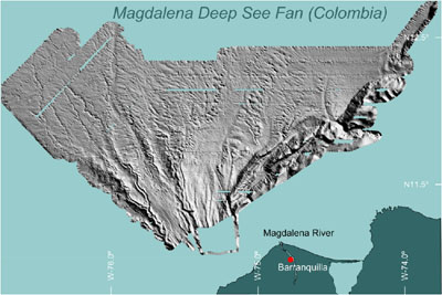
Create detailed shaded relief maps! This map shows a turbidite fan
and was created with multi-beam echo-sounder data obtained
in the Caribbean Sea
Shaded Relief Map Features
- Create photo-quality relief maps from grid files
- Control light source position, relative slope gradient, and shading
- Overlay with contour, vector, post, or base maps for highly effective displays
- Shading calculations based on several shading methods, including Simple, Peucker's Approximation, Lambertian Reflection, and Lommel-Seeliger Law
- Set relief parameters using Central Difference or Midpoint difference gradient methods
- Save and load custom color map files for the exact desired display
- Use one of the built-in presets as the color map
- Specify a color for missing data, or choose to make areas of no data transparent
- Change the rotation and tilt angles
- Adjust the layer opacity
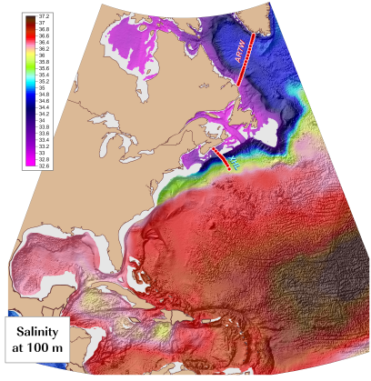
Create spectacular maps in seconds. This map consists of a shaded relief map overlaid with a contour map detailing the salinity of the Atlantic Ocean at 100 meters. Image courtesy of Igor Yashayaev, Bedford Institute of Oceanography, Canada.
Combine a shaded relief map with contour and base map features.
Post Maps
Post maps show XY locations with fixed size symbols or proportionally scaled symbols of any color.
Create post maps independent of other maps on the page, or combined with other map layers. For each posted point, specify the symbol and label type, size, and angle. Also create classed post maps that identify different ranges of data by automatically assigning a different symbol or color to each data range. Post your sample locations, well locations, or original data point locations on a contour map to show the distribution of data points on the map, and to demonstrate the accuracy of the gridding methods you use.
Use post maps to display the location of your XY data
Watershed maps
Watershed maps automatically calculate and display drainage basins and streams from your grid file.
Create colorful watershed maps to display regions draining into a stream, stream system or body of water. Display the catchment basins, streams, or both. Export the basins and streams to any supported file format, including SHP and DXF files, for use in other software! Surfer uses the accurate eight-direction pour point algorithm to calculate the flow direction at each grid node.
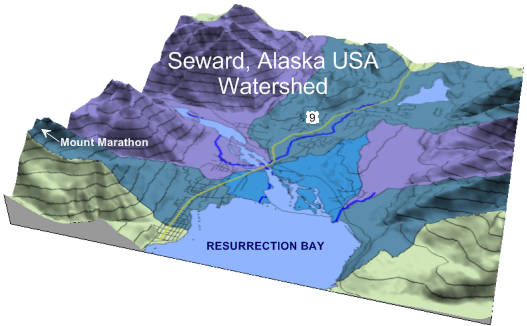
Detail every aspect of your map from creating watershed boundaries to adding city streets and
surrounding elevations, like the above map of Seward, Alaska.
- Fill the depressions, areas of internal drainage
- Save the filled grid to a new grid file
- Show streams
- Specify the threshold number of upstream cells flowing into a grid cell that are required to create a stream line
- Specify line properties for the streams
- Specify fill colors for the catchment basins
- Specify the pour point sources as stream intersections, none, or load them from a file
- Adjust the layer opacity

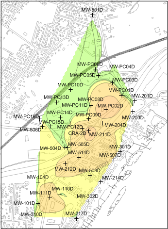
Display watershed catchment basins and streams to determine which areas
are draining into which streams.
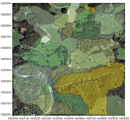
Overlay watershed maps on top of aerial photos for a complete picture!
Geobasisdaten © Bayerische Vermessungsverwaltung 2012, http://www.geodaten.bayern.de />
3D Wireframe Maps
Surfer wireframe maps provide an impressive three dimensional display of your data. Wireframes are created by connecting Z values along lines of constant X and Y. Use color zones, independent XYZ scaling, orthographic or perspective projections at any tilt or rotation angle, and different combinations of X, Y and Z lines to produce exactly the surface you want. Drape a color-filled contour map over a wireframe map to create the most striking color or black-and-white representations of your data. The possibilities are endless.
A wireframe map can be used to display any combination of X,Y, and Z lines.
A USGS SDTS DEM file was used to create this map and color zones were defined for the X and Y lines.
3D Wireframe Map Features
- Display any combination of X,Y, and Z lines
- Use automatic or user-defined color zones to highlight different Z levels
- Stack any number of 3D surfaces on a single page
- Optional hidden line removal
- Overlay any combination of contour, filled contour, base, post, and classed post maps on a surface
- Views of the top or bottom of the surface, or both
- Proportional or independent scaling in the X,Y, and Z dimensions
- Full control over axis tick marks and tick labels
- Add a base with optional vertical base lines
- Display the surface at any rotation or tilt angle
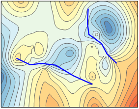
Vector maps
Instantly create vector maps in Surfer to show direction and magnitude of data at points on a map. You can create vector maps from information in one grid or two separate grids. The two components of the vector map, direction and magnitude, are automatically generated from a single grid by computing the gradient of the represented surface.
At any given grid node, the direction of the arrow points in the direction of the steepest descent. The magnitude of the arrow changes depending on the steepness of the descent. Two-grid vector maps use two separate grid files to determine the vector direction and magnitude. The grids can contain Cartesian or polar data. With Cartesian data, one grid consists of X component data and the other grid consists of Y component data. With polar data, one grid consists of angle information and the other grid contains length information. Overlay vector maps on contour or wireframe maps to enhance the presentation!
 |
 |
|
| A vector map of Mt. St. Helens overlaid on a contour map (left) and wireframe map (right). Use a color scale bar or legend to indicate the magnitude of the arrows. |
Vector Map Features
- Create vector maps based on one grid or two grids.
- Define arrow style, color, and frequency
- Symbol color may be fixed, based on vector magnitude or based on a grid file
- Save and load custom color map files for the exact desired display
- Use one of the built-in presets as the color map
- Display color scale bars and vector scale legends
- Scale the arrow shaft length, head length, and width
- Control vector symbol origin
- Choose from linear, logarithmic, or square root scaling methods
- Adjust the layer opacity
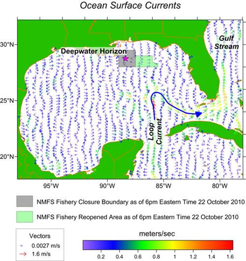
This vector map displays the ocean's surface currents. Image courtesy of
Chris Fullilove, Rip Charts.
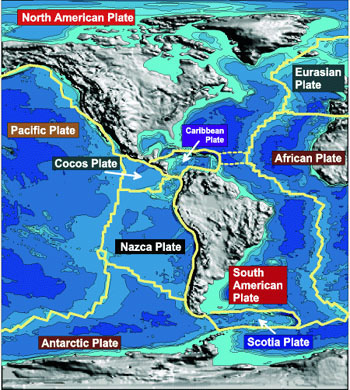
Base Maps
Surfer can import maps in many different formats to display geographic information.
Display your base maps in Surfer alone or overlay them on other maps.
Base Map Features
- Edit the line, fill, text and symbol properties for individual objects in a base map
- Globally edit the line, fill, text and symbol properties for all objects in a base map
- Import georeferenced images files in real world coordinates
- Manually georeferenced images files in real world coordinates
- Calculate the area and perimeter length of polygons in a base map
- Copy, paste, reshape, move and delete individual objects in a base map
- Add new objects to a base map
- Adjust the layer opacity
- Import, edit, export and label map features with attributes
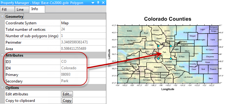
Display all your information! Attributes are imported with your base map files, or can be created. All objects in a base layer can be labeled with attributes. The polygons in this map are labeled with the Secondary attribute.
Load all your base map files to create location maps for your data!
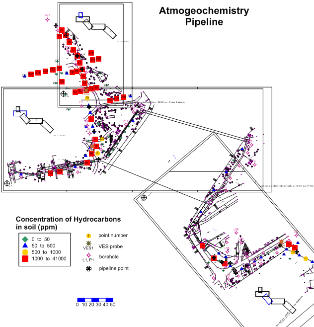
Overlay other map types, such as classed post maps, with your base map.
Map layers
Adding multiple map layers to your map gives you a way to combine different types of data in one map. For example, you can drape a georeferenced image over a 3D surface map, overlay multiple base maps with a contour map, or plot a post map with contours over a wireframe map.
And because you can add any number of map layers to a map, you can show any amount of data on a single map. You are limited only by your imagination!
 |
 |
|
| Combining surface maps is an excellent technique to visually compare data sets. | Overlay several surface maps to generate informative block diagrams. | |
 |
||
| Effortlessly produce vivid and stunning maps that display an array of data! Image courtesy of Igor Yashayaev, Bedford Institute of Oceanography, Canada. | Overlay multiple map layers and adjust the transparency of the upper layers to see the lower layers beneath! This example shows a partially transparent contour map overlaid with a georeferenced image file imported as a base map. | |
Stacking maps
You can align individual maps horizontally on the page by stacking them. Map stacking was designed to align maps using commensurate coordinate systems. This command is useful for keeping two or more maps separated vertically on the page while keeping relative horizontal positions.
Stack 2D and 3D maps to most effectively display your data
Stack and rotate maps for the best presentation possible!
Stack multiple sets of maps to display all your data!
Map Projections
Choose from an endless list of coordinate systems for your map to display. Specify the source coordinate system for each of the layers in your map, and choose to display the map in any other coordinate system! For example, load data and grid files in UTM or State Plane coordinates, and display the map in Latitude/Longitude coordinates! It is simply that easy!
Save the coordinate system information for your grid to an external file for future reuse.
This map was created using ten different data sets in more than five different
coordinate systems! No extra effort is required to convert data sets, Surfer works
seamlessly with all coordinate systems. Image courtesy of Eric Dickenson,
Environmental Science and Engineering Division, Colorado School of Mines.
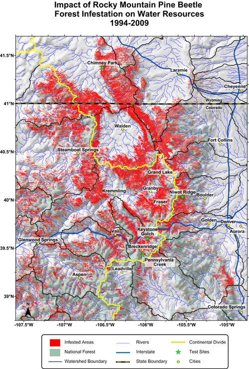
Infestation data was obtained from USDA Forest Service,
Forest Health Protection and its partners.
Profiles
Surfer's automatic profile tool makes it easy to visualize the change in Z value from one point to another.
Simply select the map, add a profile, and draw the line on the map. Include as many points as you want in the line; it could be a simple two-point line, or a zig-zag shape. In all cases, the profile is created showing the Z value change along the length of the line. Reshape the line on the map, and the profile automatically updates.
- Title and font properties
- Setting any areas with missing data to skip, minimum Z value, or a custom value
- Line and fill properties
- X and Y scaling
- Exporting the profile line to a text data file
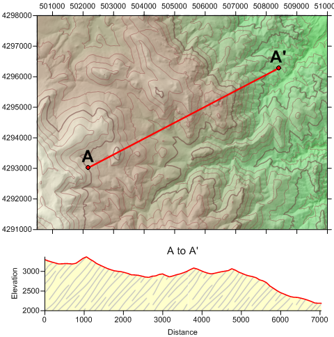
Easily create a profile by simply drawing a line on the map!
Customize Your Map
Make your map look its best by customizing it to fit your needs! Surfer offers numerous map features to enhance the look of your map. Use Surfer's defaults, or customize your map by including scale bars, editing colors, lines and fill styles, showing only portions of a map, adjusting the scale and setting axis properties!
Map Features
- Change the tilt, rotation and field of view angle for the map
- Specify the view projection as perspective or orthographic
- Set XYZ scales in map units or page length
- Choose proportional or independent XY scaling
- Display the map using the data XY limits or choose to display the map using a subset of the data
- Control background fill and line color and styles
- Full control over the axis limits and scaling, axis title, axis line style, tick labels, tick spacing, tick display, and grid lines
Other Customizations
- Create any number of maps on a single page
- Create independent maps or create a combined map with multiple types of map layers
- Add scale bars
- Add additional axes
- Add text, polylines, polygons, symbols and spline polylines
- Edit text, line, fill and symbol properties
- Set the transparency for images, fill patterns and most map layers
- Define custom line styles and colors
- Add any number of text blocks at any position on the map, using TrueType fonts
- Include superscripts, subscripts and Greek or other characters in text
- Add arrowheads to lines
Customize your map using the abundant options available to you!
Create multiple maps, scale bars, and text annotations to clarify your project.
Create the most informative maps possible by adding text, scale bars, location maps, and other details!
Superior Gridding
The gridding methods in Surfer allow you to produce accurate contour, surface, wireframe, vector, image, and shaded relief maps from your XYZ data. The data can be randomly dispersed over the map area, and Surfer's gridding will interpolate your data onto a grid. Use Surfer's default settings or choose from twelve different gridding methods.
Each gridding method provides complete control over the gridding parameters, so you can produce exactly the map you want. If your data are already collected in a regularly spaced rectangular array, you can create a map directly from your data. Computer generated contour maps have never been more accurate.
Gridding Features
- Interpolate from up to 1 billion XYZ data points (limited by available memory)
- Produce grids with up to 100 million nodes
- Specify faults and breaklines when gridding
- Choose from one of the powerful gridding methods: Inverse Distance, Kriging, Minimum Curvature, Polynomial Regression, Triangulation, Nearest
- Neighbor, Shepard's Method, Radial Basis Functions, Natural Neighbor, Moving Average, and Local Polynomial
- Specify isotropic or anisotropic weighting
- You have full control over the grid line geometry including grid limits, grid spacing, and number of grid lines
- Customize search options based on user-defined data sector parameters
- Specify search ellipses at any orientation and scaling
- Use spline smoothing and grid filtering to alter the grid file
- Use grid math to perform mathematic operations between grid files
- Use Nearest Neighbor to create grid files without interpolation
- Use Triangulation to achieve accuracy with large data sets faster
- Detrend a surface using Polynomial Regression, generate regression coefficients in a report, and calculate residuals
- Use data exclusion filters to eliminate unwanted data
- Use duplicate data resolution techniques
- Generate a grid of Kriging standard deviations
- Specify point or block Kriging
- Generate a report of the gridding statistics and parameters including ANOVA regression statistics
- Specify scales and range for each variogram model
- Generate grids from a user-specified function of two variables
- Calculate grids with Data Metrics including: number of points within search ellipse, distance to nearest and farthest neighbor, median, average and offset distance to points within the search ellipse
- Use cross-validation to judge the suitability of the gridding method for the particular data set
- Save grid files in these formats: ADF, AGR, AIG, AM, ASC, BIL, BIN, BIP, BSQ, COL, DAT, DEM, ERS , FLD, FLT, GGF, GRD, GXF, HDF,IMG, LAT, RAW, and VTK
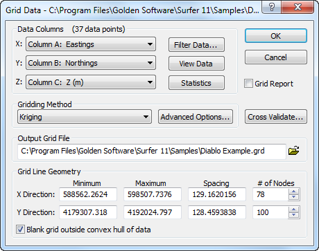
Set the gridding parameters in the Grid Data dialog.
Grid Node Editor
Clean up your grid with the grid node editor!
Surfer's powerful grid node editor allows you to view and edit each individual grid node in a grid file. You can edit the grid node's Z value simply by selecting a grid node and entering a new Z value in the edit box. Grid nodes are represented by small black +'s, and blanked nodes (null values) are represented by blue x's, so it is easy to see your exact data.
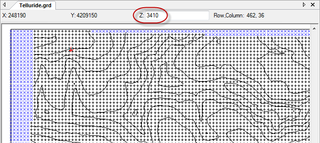
Select a grid node and the Z value for that node is displayed in the toolbar.
You can edit the Z value and resave the grid.
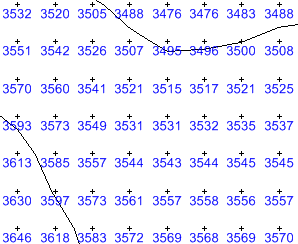
Zoom in close to the grid nodes and the Z value for each
grid node is displayed under the symbol!
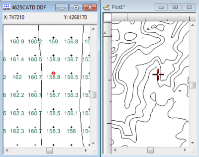
Track the grid node location on a map by clicking
on a node in the grid node editor window, and having the
respective location highlighted on the map in the plot window.
Variograms
Use the variogram modeling subsystem to quantitatively assess the spatial continuity of data. Variograms may be used to select an appropriate variogram model when gridding with the Kriging algorithm. Surfer uses a variogram grid as a fundamental internal data representation and once this grid is built, any experimental variogram can be computed instantaneously.
Instantly create variograms in Surfer to quantitatively
assess the spatial continuity of your data.
Variogram Features
- Virtually unlimited data set sizes
- Display both the experimental variogram and the variogram model
- Specify the estimator type: variogram, standardized variogram, auto covariance, or auto correlation
- Specify the variogram model components: exponential, Gaussian, linear, logarithmic, nugget effect, power, quadratic, rational quadratic, spherical, wave, pentaspherical, and cubic models
- Customize the variogram to display symbols, variance, and number of pairs for each lag
- Export the experimental variogram data
- Download variogram tutorial
Faults and Breaklines
Define faults and breaklines when gridding your data. Faults act as barriers to the information flow, and data on one side of the fault will not be directly used to calculate grid node values on the other side of the fault. Breaklines include Z values.
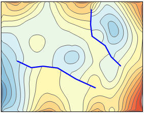
When Surfer sees a breakline, it uses the Z value of the breakline in combination with nearby data points to calculate the grid node value. Unlike faults, breaklines are not barriers to information flow and the gridding algorithm can cross the breakline to use a point on the other side to calculate a grid node value. Use breaklines to define streamlines, ridges, and other breaks in slopes.
The gridding methods that support faults are: Inverse Distance to a Power, Minimum Curvature, Nearest Neighbor, and Data Metrics.
The gridding methods that support breaklines are: Inverse Distance to a Power, Kriging, Minimum Curvature, Nearest Neighbor, Radial Basis Function, Moving Average, Data Metrics, and Local Polynomial.
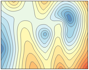 Original contour map without faults or breaklines. |
||
 |
 |
|
| The same data set gridded with two breaklines and displayed as a contour map. |
The same data set gridded with two breaklines and displayed as a contour map. |
|
Grid Functions
In addition to creating maps, you can perform a variety of functions using grid files. Just a few of the possibilities include:
- Calculating the volume and areas of grid files! You can calculate the planar and surface area, and calculate the volume between two files, or a grid file and any horizontal plane.
- Applying a mathematical equation to grid files. Examples include subtracting one grid file from another to create an isopach map, converting outliers to a minimum or maximum value, or multiplying one grid file by a conversion factor to convert the Z units from meters to feet.
- Applying grid filters to emphasize details or remove background variation in the grid file.
- Blanking specified regions in a grid file to prevent contours or map data from being drawn through those areas (ie. buildings, roads, or outside of field areas).
- Creating cross sections and topographical profiles.
- Combining multiple grid files into a single, easy to use grid file.
- Extracting subsets of grids or DEMs based on rows and columns.
- Transforming, offset, rescale, rotate, and mirror grids.
- Smoothing grid files to create smoother maps.
- Calculating first and second directional derivatives at user-specified orientations.
- Calculating differential and integral operators utilizing gradient, Laplacian, biharmonic, and integrated volume operators.
- Analyzing your data with Fourier and Spectral Analysis with Correlograms and Periodogram.
- Calculating residuals to find the difference between the original data point values the interpolated Z values at those points, or to find the Z values at any specific XY locations.
- Converting a grid file from any supported format to any other supported format.
- Last 10 grid functions are automatically saved.
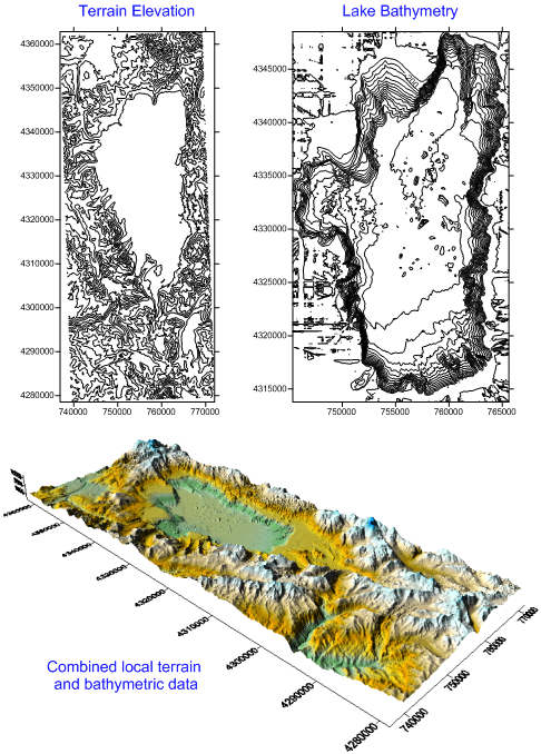
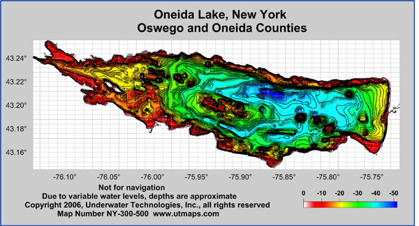
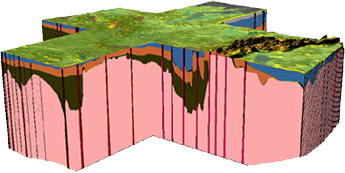
Grid functions were used to combine bathymetric data with local terrain data.
Available grid functions in Surfer converted the Z values in the bathymetric grid from
bathymetric units to elevation units, and cleared the data in the areas outside the
lake boundary. The grid of lake bathymetry was then combined with the grid of
the local terrain elevation to create a single composite grid file.
Use USGS Digital Elevation Model (DEM), National Elevation Dataset (NED) and NASA Shuttle Radar Topographic Mission (SRTM) data with any Surfer command that uses grid files.
- Directly use the files in native format without modification or conversion.
- Display information about the files, such as X, Y and Z extents or grid statistics.
- Create contour, vector, shaded relief, image, 3D surface, and 3D wireframe maps from the files.
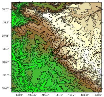
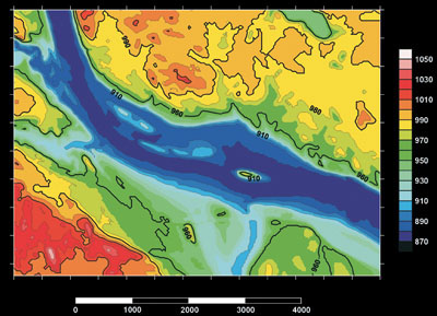
The above contour map was generated from a grid file in BIL format,
downloaded from the USGS The National Map Seamless Server
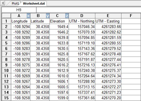
Worksheet
Surfer lets you massage your data in many ways to achieve the exact output you want. Surfer includes a full-featured worksheet for creating, opening, editing, and saving data files. Data files can be up to one billion rows and columns, subject to available memory. You can cut, copy, and paste data within the Surfer worksheet or between applications.
Worksheet Features
- Import a database directly into the Surfer worksheet
- Calculate data statistics
- Perform data transformations using advanced mathematical functions
- Sort data based on primary and secondary columns
- Spatially filter data
- Assign a projection or coordinate system to your data, and convert the data to a new projection or coordinate system
- Select a predefined coordinate system from Geographic (lat/lon) or one of the supported projected systems (Polar/Arctic/Antarctic, Regional/National, State Plane, UTM, and World)
- Define a custom coordinate system by selecting a supported projection, specifying the projection settings, and either choosing one of over 400 predefined datums or creating a custom datum
- Add a frequently used coordinate system to the Favorites list to be easily accessible
- Assign which columns in the worksheet contain the X, Y and Z data
- Use the Find/Replace function in the worksheet to easily find or replace your data
- Print the worksheet
Object and Property Manager
The object manager and property manager makes the editing of any object simple. The object manager displays all the objects in the plot document in an easy-to-use hierarchical tree arrangement.
Double click on objects in the object manager to easily edit them, check or uncheck the check boxes next to their name to show or hide them, drag and drop objects to rearrange the order in which they are drawn, and overlay maps by dragging and dropping map layers from one map frame into another! Select any object or map layer in the object manager for easy deletion.
When an object is selected in the object manager, changes to the object can be made in the property manager. The property manager is a docked window that is always displayed on the screen. You can make the property manager floating or close it, if you do not want it to display. All of the properties for an object are listed in the property manager. For instance, the Contours layer is selected in the object manager in the image below, and you can change the contour layer properties in the property manager. Once the change is made in the property manager, it is immediately applied in the plot window.
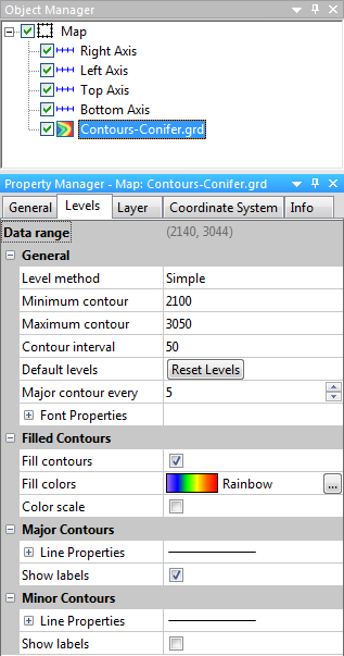
Use the object manager and property manager
to easily access and edit all objects
in your plot window.
Create your own scripts to automate repetitive tasks! Don't spend time doing the same process over and over again – write a simple script to simplify your life! Operations performed interactively can be controlled using an automation-compatible programming language such as Visual Basic, C++, or Perl.
Surfer includes Scripter, a built-in Visual Basic compatible programming environment that lets you write, edit, debug, and run scripts. Why do more work than you need when you have Surfer working for you!
Visit the Support Central page where you'll find over 35 sample scripts to help you get started.
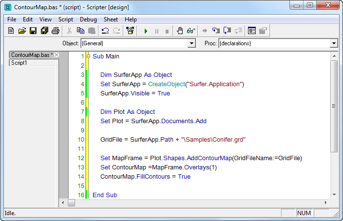
Write simple scripts to call repetitive tasks
Additional Features
Your Surfer package comes with many additional features to help you work smarter, not harder!
- Reload map data and grid files with a single command
- Draw a polyline or polygon to measure distance and area
- Use the Text Editor to easily format, superscript, subscript and edit text or insert symbols or equations
- Edit boundary files by converting between polylines and polygons, combining and splitting islands/lakes, and connecting and breaking polylines
- Substitute a new grid or data file into an existing map without changing the map properties
- Save a grid from a grid-based map, or save a data file from a post or classed post map.
- Display the XYZ coordinates of the cursor location in the status bar
- Windows Clipboard support for copying maps to other applications
- Use the mouse to resize objects on the screen
- Define Surfer's default preferences
- Easily find XYZ coordinates by digitizing point locations
- Automatically save digitized coordinates as BLN or ASCII data files
- Print to any Windows supported printer or plotter
- Display and print subsets of completed maps, complete with subset axes
- Adjust the number of Undo levels
- Use the reshape tool to edit areas and curves
- Click on a map and pinpoint the same XY location in a different map
- Click on a map and highlight the nearest data point to that location in the worksheet
- Create your own keyboard shortcuts for common functions
- Customize the toolbars by adding or removing buttons
- Floatable toolbars
- Download free updates automatically
- Install the 32-bit or 64-bit version of Surfer
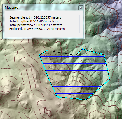
Use the Measure tool to draw a region over the map and
measure the length and area of the region!
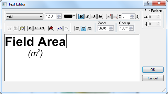
Use the Text Editor to easily create and edit custom text.
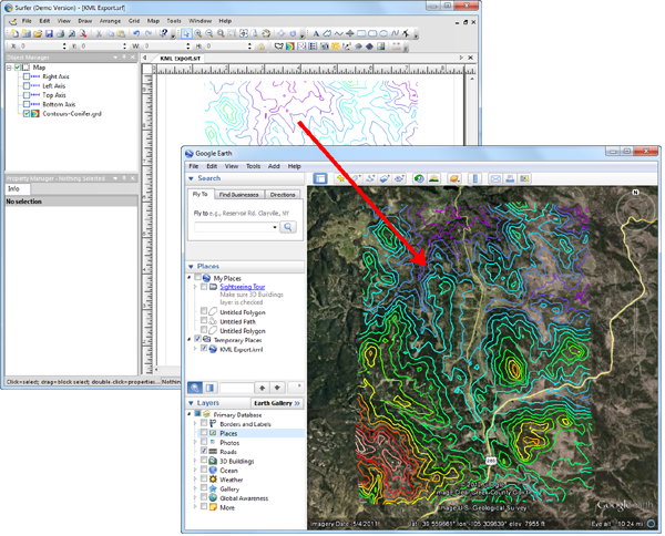
Export your map in KML or KMZ format for convenient display in Google Earth!
Supported File Format
Surfer 10 supports many data, grid, and import/export formats.
| DATA FILES | GRID FILES | EMPORT / EXPORT |
Open Data: Save Data: |
Open Grids: Save Grids: |
Import: Export: |